When a conditional formatting rule is overkill, use these VBA procedures to highlight duplicates and then remove the highlighting in Microsoft Excel.

Image: Rawpixel.com/Shutterstock
There are many ways to find duplicates in a Microsoft Excel data range—conditional formatting being one of the most commonly used. When the rule is TRUE, the format stays until the condition is FALSE or you remove the rule. However, sometimes, you only want a quick look or count of duplicates; you don’t want a permanent format. Or, more reasonably, users might not be savvy enough to apply a conditional formatting rule. In either case, this article will review VBA code that highlights duplicates in a data range. This article also includes code to remove highlighting from a data range.
SEE: 83 Excel tips every user should master (TechRepublic)
I’m using Microsoft 365 on a Windows 10 64-bit system, but you can use earlier versions. Use the downloadable .xlsm, .xls, or .cls files to obtain the code. Excel Online doesn’t support macros. This article assumes that you have basic Excel skills; however, even a beginner should be able to follow the instructions to success.
How to use the VBA procedure
Before we review the procedures, it’s worth noting that code-wise, the two procedures are almost identical. You could combine the two into one procedure and prompt the user to identify whether the task is to highlight or remove highlighting, but that requires an extra click every time you run the procedure. Running two eliminates that extra click. But some would choose to combine them, so it’s worth considering.
Listing A highlights duplicate values in a data range. After declaring and defining variables, the code prompts the user to select a range. After checks on that selection, the code highlights duplicates and then displays the number of duplicates highlighted. Listing B is similar but removes highlights and doesn’t display the duplicate count.
HighlightDuplicates() sets a highlight by setting the ColorIndex property to 36, which is yellow; Listing B sets the same setting to 0, which is no fill color at all. If the range has a permanent fill color, you’ll want to accommodate that in Listing B by using that same fill color setting instead of 0.
Listing A
Sub HighlightDuplicates()
‘Highlight duplicates in selected range.
Dim selRange As Range
Dim curCell As Range
Dim j As Integer
‘Prompt user to select range.
‘Must have Break on Unhandled Errors selected.
On Error Resume Next
Set selRange = Application.InputBox( _
Title:=”Select range”, _
Prompt:=”Select a range to check for duplicate values.”, _
Type:=8)
On Error GoTo 0
‘Test for cancel.
If selRange Is Nothing Then Exit Sub
‘Test for single-cell selection.
If selRange.Rows.Count = 1 Then
MsgBox “You’ve selected only one cell. ” _
& “Please select multiple contiguous cells ” _
& “within a single column.”, vbOKOnly
Exit Sub
End If
‘Set counter to 0.
j = 0
‘Cycle through user-selected range to highlight duplicates.
For Each curCell In selRange
If WorksheetFunction.CountIf(selRange, curCell.Value) > 1 Then
curCell.Interior.ColorIndex = 36
j = j + 1
End If
Next curCell
j = j / 2
MsgBox “You have ” & j & ” duplicates.”, vbOKOnly
End Sub
Listing B
Sub DeleteDuplicates()
‘Highlight duplicates in selected range.
Dim selRange As Range
Dim curCell As Range
‘Prompt user to select range.
‘Must have Break on Unhandled Errors selected.
On Error Resume Next
Set selRange = Application.InputBox( _
Title:=”Select range”, _
Prompt:=”Select a range to check for duplicate values.”, _
Type:=8)
On Error GoTo 0
‘Test for cancel.
If selRange Is Nothing Then Exit Sub
‘Test for single-cell selection.
If selRange.Rows.Count = 1 Then
MsgBox “You’ve selected only one cell. ” _
& “Please select multiple contiguous cells ” _
& “within a single column.”, vbOKOnly
Exit Sub
End If
‘Cycle through user-selected range to highlight duplicates.
For Each curCell In selRange
If WorksheetFunction.CountIf(selRange, curCell.Value) > 1 Then
curCell.Interior.ColorIndex = 0
End If
Next curCell
End Sub
If you’re using a ribbon version, be sure to save the workbook as a macro-enabled file or the procedure won’t run. If you’re using a menu version, you can skip this step.
SEE: Windows 10: Lists of vocal commands for speech recognition and dictation (free PDF) (TechRepublic)
To enter both procedures, press Alt + F11 to open the Visual Basic Editor. In the Project Explorer to the left, select ThisWorkbook so you can run the procedure in any sheet. You can enter the code manually or import the downloadable .cls file. In addition, the macro is in the downloadable .xlsm and .xls files. If you enter the code manually, don’t paste from this web page. Instead, copy the code into a text editor and then paste that code into the ThisWorkbook module. Doing so will remove any phantom web characters that might otherwise cause errors.
Use the procedures
After entering the procedures, you’re ready to put them to work as follows:
- Click the Developers tab.
- Click Macros in the Code group.
- In the resulting dialog, choose HighlightDuplicates() as shown in Figure A and click Run.
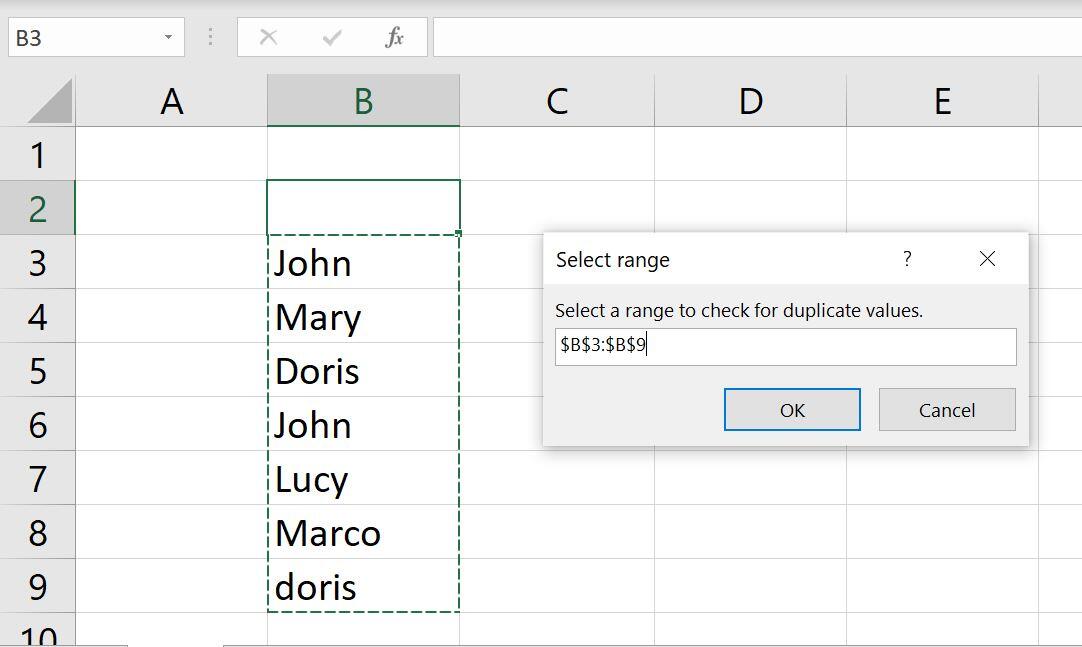
- When prompted, select B3:B9 as shown in Figure B, and click OK.
- Click OK to close the information message that displays the number of duplicates, shown in Figure C.
Figure A
” data-credit>
This procedure highlights duplicate values.
Figure B
” data-credit>
Select the range you’re checking for duplicates.
Figure C
” data-credit>
The counting variable tracks the number of duplicates.
That’s it! As you can see in Figure C, the procedure found two duplicates. Those four cells are now yellow, which means two values have a duplicate: John and Doris. Notice that the code isn’t case sensitive (Doris and doris).
The On Error statements catch keystrokes instead of a range selection. The For-loop cycles through each cell in the selected range and applies a highlight when the expression
WorksheetFunction.CountIf(selRange, curCell.Value) > 1
is TRUE, meaning the current value occurs more than once in the data set. The COUNTIF() function is the same you’d use if creating a conditional formatting rule. The last thing the procedure does is display the number of duplicate values, in this case, that’s two.
Next, run DeleteHighlights(), select the same range and the procedure will quickly remove the highlights. Both procedures check for a Cancel click and a single-cell range.
Things to consider
Both procedures are fairly flexible. They evaluate text, numbers, and dates, even if they’re in the same data range. They both work with multiple columns, evaluating all the entries as a whole. In other words, the code finds duplicates in the same column as well as duplicates shared across multiple columns. The code ignores blanks and isn’t case-sensitive.
You could make the process more dynamic by grabbing the fill color before applying the highlighting in Listing A and saving it as a static variable that maintains its value. Listing B could then reference that variable and use it to reset the cell’s fill color when removing highlighting.
It’s unlikely that you’ll want to work through all those steps every time you want to run the procedure. Instead, add the macro to the Quick Access Toolbar. To do so, read How to add Office macros to the QAT toolbar for quick access.
Also see
Source of Article


